Boundary conditions

Finite-difference and WENO stencils reach beyond the mesh near its borders; a boundary condition supplies the missing ghost values. The following are available:

ExtrapolationBC{P} uses the P+1 nearest interior cells to build a degree-P polynomial and extrapolates it into the ghost region; higher P gives smoother outflow at the cost of a wider stencil.

Specifying conditions per face

When constructing a level-set equation you can pass up to $2d$ boundary conditions, one per face, where $d$ is the dimension. The convention is:

• a single boundary condition is applied to all $2d$ faces;
• a length-$d$ collection bcs assigns bcs[i] to direction i, and there bcs[i] may be
  • a single condition, applied to both faces of direction i, or
  • a tuple (lo, hi) of two conditions, applied to the lower/left and upper/right face.

Periodic vs. open boundaries

The clearest way to see what a condition does is to watch the same flow leave the domain under different boundaries. We advect a disk to the right with $\boldsymbol u = (1, 0)$: a PeriodicBC wraps it back in from the left, while a NeumannBC lets it flow out cleanly.

using LevelSetMethods, GLMakie
LevelSetMethods.set_makie_theme!()
grid = CartesianGrid((-1, -1), (1, 1), (48, 48))
ϕ₀ = MeshField(x -> sqrt(x[1]^2 + x[2]^2) - 0.5, grid)
𝐮 = AdvectionTerm((x, t) -> (1, 0))

eq_periodic = LevelSetEquation(; ic = ϕ₀, bc = PeriodicBC(), terms = 𝐮)
eq_open     = LevelSetEquation(; ic = ϕ₀, bc = NeumannBC(),  terms = 𝐮)

fig = Figure(; size = (1000, 480))
for (n, t) in enumerate((0.0, 0.5, 0.75, 1.0))
    integrate!(eq_periodic, t)
    integrate!(eq_open, t)
    ax1 = Axis(fig[1, n]; title = "periodic, t = $t")
    plot!(ax1, eq_periodic)
    ax2 = Axis(fig[2, n]; title = "open (Neumann), t = $t")
    plot!(ax2, eq_open)
end
fig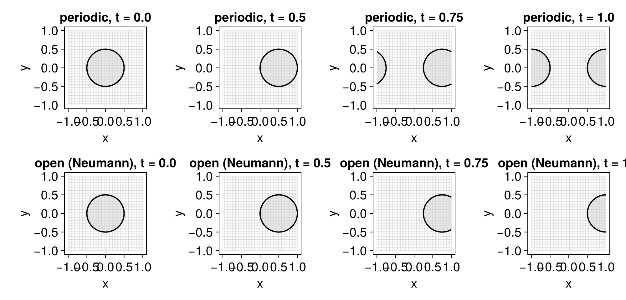

For higher-order outflow, use ExtrapolationBC{P} directly: ExtrapolationBC(5), say, fits a degree-5 polynomial through the 6 nearest interior cells. Higher P smooths the extrapolation into the ghost region at the cost of a wider stencil; for plain outflow like the above it behaves much like NeumannBC.

Mixing conditions

Pass a per-direction tuple to combine conditions — here open in x, periodic in y, under a diagonal flow $\boldsymbol u = (1, 1)$:

bc = (NeumannBC(), PeriodicBC())   # Neumann in x, periodic in y
eq = LevelSetEquation(; ic = ϕ₀, bc, terms = AdvectionTerm((x, t) -> (1, 1)))
fig = Figure(; size = (1000, 280))
for (n, t) in enumerate((0.0, 0.5, 0.75, 1.0))
    integrate!(eq, t)
    ax = Axis(fig[1, n]; title = "t = $t")
    plot!(ax, eq)
end
fig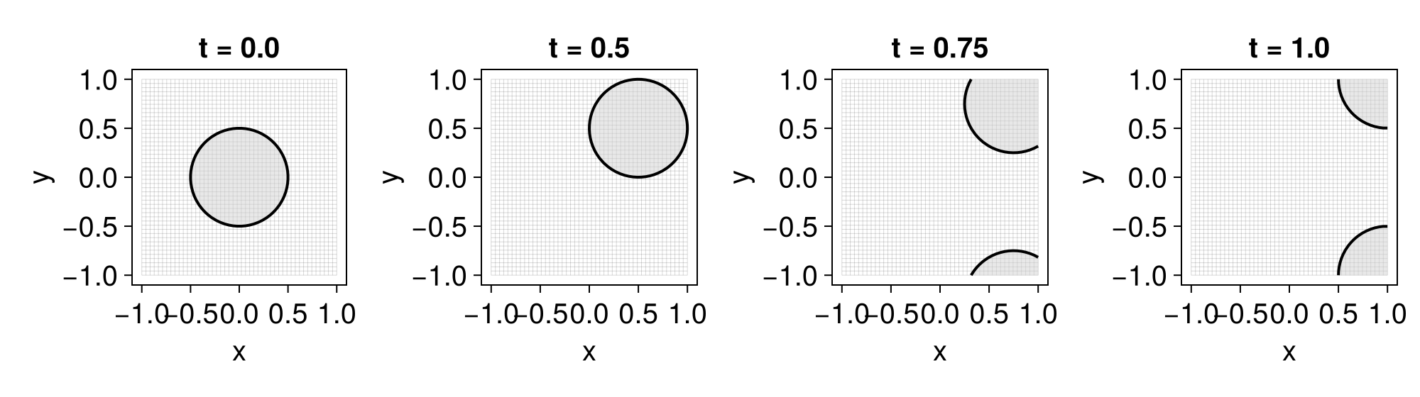

Symmetry planes

A SymmetryBC treats a boundary as a mirror: the field is reflected across it, so the interface meets the boundary perpendicularly. Like NeumannBC it enforces $\partial\phi/\partial n = 0$, but by reflection rather than flat extension — exactly the condition that holds on the axis of a symmetric problem. That lets you simulate only half of such a problem and recover the rest by reflection.

Below we stretch a disk centred on the axis $x = 0$ by the symmetric strain flow $\boldsymbol{u} = (x, 0)$, solving it twice: on the full domain, and on the right half with a SymmetryBC on the axis. We overlay the two — full solution solid, half solution a dashed red contour, axis $x = 0$ dotted. The recipe forwards standard Makie attributes (color, linestyle, linewidth, and a fill toggle for the interior shading), which is what lets the half solution be drawn as a bare contour on top of the full one:

𝐯 = (x, t) -> (x[1], 0.0)   # symmetric about x = 0 (uₓ is odd in x)
ic(g) = MeshField(x -> hypot(x...) - 0.4, g)

grid_full = CartesianGrid((-1.0, -1.0), (1.0, 1.0), (40, 40))
grid_half = CartesianGrid(( 0.0, -1.0), (1.0, 1.0), (20, 40))   # right half only
eq_full = LevelSetEquation(; ic = ic(grid_full), bc = NeumannBC(), terms = AdvectionTerm(𝐯))
# SymmetryBC on the axis face (x = 0) only; Neumann on the remaining faces
eq_half = LevelSetEquation(; ic = ic(grid_half), bc = ((SymmetryBC(), NeumannBC()), NeumannBC()), terms = AdvectionTerm(𝐯))

fig = Figure(; size = (1000, 340))
for (n, t) in enumerate((0.0, 0.3, 0.6))
    integrate!(eq_full, t)
    integrate!(eq_half, t)
    ax = Axis(fig[1, n]; title = "t = $t")
    plot!(ax, eq_full; color = :crimson, linestyle = :dash)
    plot!(ax, eq_half; fill = false, showgrid = false)
    vlines!(ax, [0.0]; color = (:black, 0.4), linestyle = :dot)     # the symmetry axis
end
fig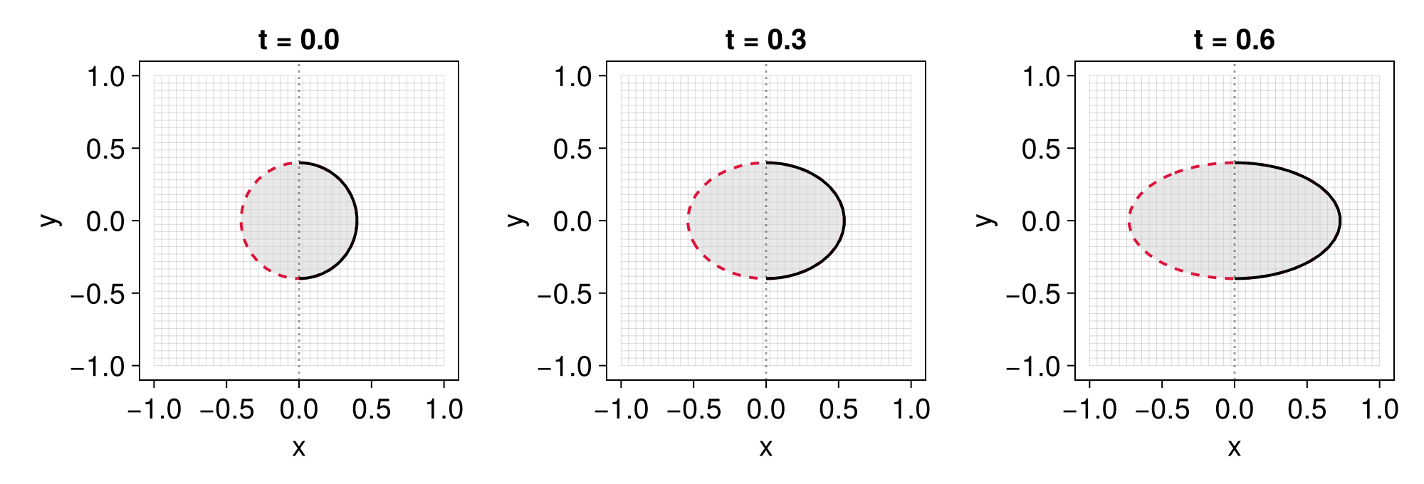

At every instant the dashed half-domain interface lies on the right half of the solid full-domain one: the SymmetryBC reproduces the symmetric solution from half the domain — the missing left half being just its mirror image — at half the computational cost.

For the precise stencil each condition applies, see the docstring of the corresponding type.