Blur & Roberts image filters
![]()
This example illustrate the use of DataFlowTasks.jl to parallelize the tiled application of two kernels used in image processing. The application first applies a blur filter on each pixel of the image; in a second step, the Roberts cross operator is applied to detect edges in the image.
Let us first load a test image:
using Images
url = "https://upload.wikimedia.org/wikipedia/commons/c/c3/Equus_zebra_hartmannae_-_Etosha_2015.jpg"
ispath("test-image.jpg") || download(url, "test-image.jpg")
img = Gray.(load("test-image.jpg"))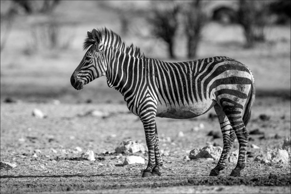
We start by defining a few helper functions:
the
contractandexpandfunctions manipulate ranges of indices in order to respectively contract or expand them by a few pixels;the
img2matandmat2imgconvert between a Gray-scale image and a matrix of floating-point pixel intensities. The filters will work on this latter representation, which may need a renormalization to be converted back to a Gray-scale image.
contract(range,n) = range[begin+n:end-n]
expand(range,n)   = range[begin]-n:range[end]-n

function img2mat(img)
    PixelType = eltype(img)
    mat = Float64.(img)
    return (PixelType, mat)
end

function mat2img(PixelType, mat)
    m1, m2 = extrema(mat)
    PixelType.((mat .- m1) ./ (m2-m1))
end

PixelType, mat = img2mat(img);
Filters implementation
The blur! function averages the value of each pixel with the values of all pixels less than width pixels away in manhattan distance. In order to simplify the implementation, the filter is applied only to pixels that are sufficiently far from the boundary to have all their neighbors correctly defined.
Results are written in-place in a pre-allocated dest array. Unless otherwise specified, the filter is applied to the whole image, but can be reduced to a tile if a smaller range argument is provided.
function blur!(dest, src; range=axes(src), width)
    ri, rj = intersect.(range, contract.(axes(src), width))

    weight = 1/(2*width+1)^2
    @inbounds for i in ri, j in rj
        dest[i,j] = 0
        for δi in -width:width, δj in -width:width
            dest[i,j] += src[i+δi, j+δj]
        end
        dest[i,j] *= weight
    end
end
blur! (generic function with 1 method)In the following, we'll use a filter width of 5 pixels, which produces the following results on the test image:
width = 5
blurred = zero(mat)

blur!(blurred, mat; width)

mat2img(PixelType, blurred)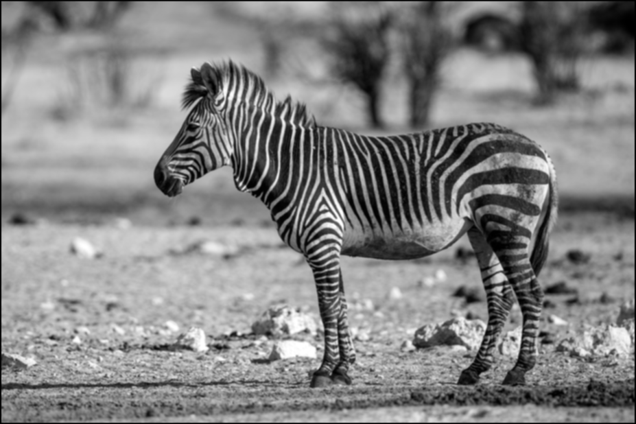
The roberts! function applies the Roberts cross operator to the provided image. Like above, it operates by default on all pixels in the image (provided they are sufficiently far from the boundaries), but can be restricted to work on a tile if the range argument is provided.
function roberts!(dest, src; range=axes(src))
    ri, rj = intersect.(range, contract.(axes(src), 1))

    for i in ri, j in rj
        dest[i,j] = (
            + (sqrt(src[i,  j]) - sqrt(src[i+1,j+1]))^2
            + (sqrt(src[i+1,j]) - sqrt(src[i  ,j+1]))^2
        )^(0.25)
    end
end
roberts! (generic function with 1 method)Applying this edge detection filter on the original image produces the following results:
contour = zero(mat)
roberts!(contour, mat)

mat2img(PixelType, contour)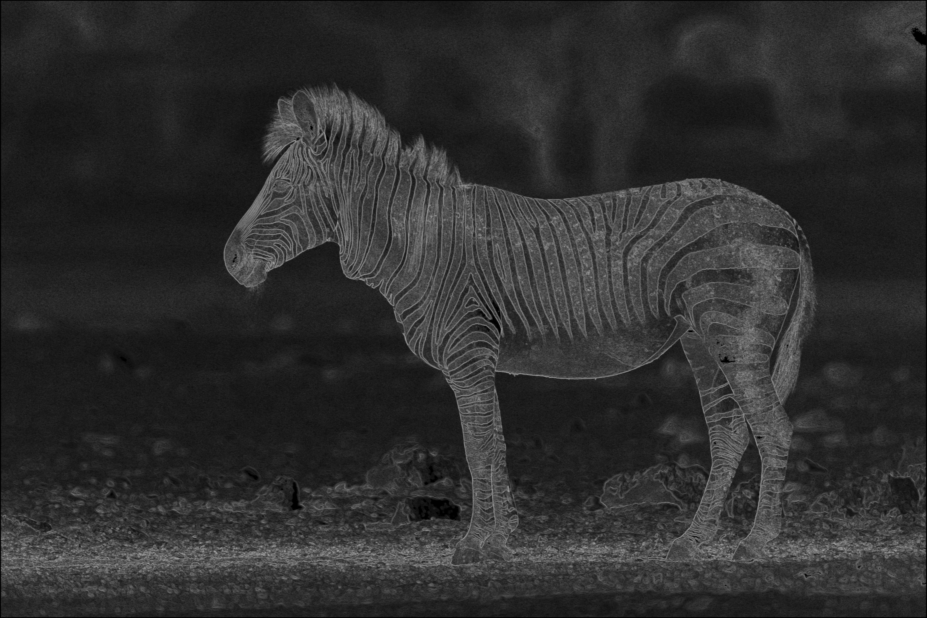
Chaining the blur and roberts filters may make edge detection less noisy:
function blur_roberts!(img; width, tmp=zero(img))
    blur!(tmp, img; width)
    roberts!(img, tmp)
end

mat1 = copy(mat)
tmp  = zero(mat)

blur_roberts!(mat1; width, tmp)
mat2img(PixelType, mat1)
The elapsed time in this sequential version will serve as reference to evaluate the performance of other implementations:
using BenchmarkTools
t_seq = @belapsed blur_roberts!(x, width=$width, tmp=$tmp) setup=(x=copy(mat)) evals=12.029620097Tiled filter application
The TiledIteration.jl package implements various tools allowing to define and iterate over disjoint tiles of a larger array. We'll use it to apply the filters tile by tile.
The map_tiled! higher-order function automates the application of a filter fun! on all pixels of an image src decomposed with a tilesize ts. This higher-order function is then used to define tiled versions of the blur and roberts filters.
using TiledIteration

function map_tiled!(fun!, dest, src, ts)
    for tile in TileIterator(axes(src), (ts, ts))
        fun!(dest, src, tile)
    end
end

blur_tiled!(dest, src, ts; width) = map_tiled!(dest, src, ts) do dest, src, tile
    blur!(dest, src; width, range=tile)
end

roberts_tiled!(dest, src, ts) = map_tiled!(dest, src, ts) do dest, src, tile
    roberts!(dest, src; range=tile)
end

function blur_roberts_tiled!(img, ts; width, tmp=zero(img))
    blur_tiled!(tmp, img, ts; width)
    roberts_tiled!(img, tmp, ts)
end
blur_roberts_tiled! (generic function with 1 method)Decomposing the original image in tiles of size $512\times 512$, the tiled application of the filters yields the same result as above:
ts = 512

mat1 .= mat
blur_roberts_tiled!(mat1, ts; width, tmp)

mat2img(PixelType, mat1)
Depending on the system, the fact that memory is now accessed in blocks may (or may not) have a significant impact on the performance, due to cache effects.
t_tiled = @belapsed blur_roberts_tiled!(x, ts; width=$width, tmp=$tmp) setup=(x=copy(mat)) evals=11.911821708Parallel filter application
Parallelizing the tiled filter application is relatively straightforward using DataFlowTasks.jl. As usual, it involves specifying which data is accessed by each task.
using DataFlowTasks

function blur_dft!(dest, src, ts; width)
    map_tiled!(dest, src, ts) do dest, src, tile
        outer = intersect.(expand.(tile, width), axes(src))
        @dspawn begin
            @R view(src, outer...)
            @W view(dest, tile...)
            blur!(dest, src; width, range=tile)
        end label="blur ($tile)"
    end
    @dspawn @R(dest) label="blur (result)"
end

function roberts_dft!(dest, src, ts)
    map_tiled!(dest, src, ts) do dest, src, tile
        outer = intersect.(expand.(tile, 1), axes(src))
        @dspawn begin
            @R view(src, outer...)
            @W view(dest, tile...)
            roberts!(dest, src; range=tile)
        end label="roberts ($tile)"
    end
    @dspawn @R(dest) label="roberts (result)"
end
roberts_dft! (generic function with 1 method)Note how each filter spawns one task for each tile, and an extra task to get the results in the end. This allows applying a given filter independently of the other.
However, the filters remain composable: when applying both filters one after the other, no implicit synchronization is enforced at the end of the blurring stage, and the runtime may decide to intersperse blurring and roberts tasks (as long as the blurring of a tile and all its neighbors is performed before the application of the roberts filter on this tile).
function blur_roberts_dft!(img, ts; width, tmp=zero(img))
    blur_dft!(tmp, img, ts; width)
    roberts_dft!(img, tmp, ts)
    @dspawn @R(img) label="result"
end
blur_roberts_dft! (generic function with 1 method)Again this yields the same results on the test image:
mat1 .= mat;
blur_roberts_dft!(mat1, ts; width, tmp) |> wait

mat2img(PixelType, mat1)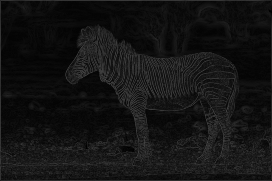
t_dft = @belapsed wait(blur_roberts_dft!(x, ts; width=$width, tmp=$tmp)) setup=(x = copy(mat)) evals=10.303081187Performance analysis
DataFlowTasks.stack_weakdeps_env!()
using CairoMakie

barplot([t_seq, t_tiled, t_dft],
        axis = (; title = "Elapsed time [s]",
                xticks=(1:3, ["sequential", "tiled", "DataFlowTasks"])))
A comparison of the performances of all implementations shows that the DataFlowTasks-based implementation produces a good speedup:
(;
 nthreads = Threads.nthreads(),
 speedup = t_seq / t_dft)
(nthreads = 8, speedup = 6.696621842780364)We can gain more insight by collecting profiling data:
GC.gc()
mat1 .= mat;
log_info = DataFlowTasks.@log wait(blur_roberts_dft!(mat1, ts; width, tmp))
DataFlowTasks.describe(log_info)
• Elapsed time : 0.319
├─ Critical Path : 0.081
╰─ No-Wait : 0.288
• Run time : 2.550
├─ Computing : 2.302
│ ╰─ unlabeled : 2.302
├─ Task Insertion : 0.001
╰─ Other (idle) : 0.248The parallel trace shows how blur and roberts tasks are interspersed in the time line:
trace = plot(log_info, categories=["blur", "roberts"])
This page was generated using Literate.jl.