Debugging & Profiling

DataFlowTasks defines two visualization tools that help when debugging and profiling parallel programs:

• a visualization of the Directed Acyclic Graph (DAG) internally representing task dependencies;
• a visualization of how tasks were scheduled during a run, alongside with other information helping understand what limits the performances of the computation.

Let's first introduce a small example that will help illustrate the features introduced here:

using DataFlowTasks

# Utility functions
init!(x)    = (x .= rand())     # Write
mutate!(x)  = (x .= exp.(x))    # Read+Write
result(x,y) = sum(x) + sum(y)   # Read

# Main work function
function work(A, B)
    # Initialization
    @dspawn init!(@W(A))               label="init A"
    @dspawn init!(@W(B))               label="init B"

    # Mutation
    @dspawn mutate!(@RW(A))            label="mutate A"
    @dspawn mutate!(@RW(B))            label="mutate B"

    # Final read
    res = @dspawn result(@R(A), @R(B)) label="read A,B"
    fetch(res)
end

work (generic function with 1 method)

Creating a LogInfo

In order to inspect code which makes use of DataFlowTasks, you can use the DataFlowTasks.@log macro to keep a trace of the various parallel events and the underlying DAG. Note that to avoid profiling the compilation time, it is often advisable to perform a "dry run" of the code first, as done in the example below:

# Context
A = ones(2000, 2000)
B = ones(3000, 3000)

# precompilation run
work(copy(A),copy(B))

# activate logging of events
log_info = DataFlowTasks.@log work(A, B)

LogInfo with 5 logged tasks

The log_info object above, of LogInfo type, contains information that can be used to reconstruct both the inferred task dependencies, and the parallel execution traces of the DataFlowTasks. A summary of this information can be displayed using DataFlowTasks.describe, as illustrated next:

DataFlowTasks.describe(log_info; categories=["init", "mutate", "read"])

• Elapsed time           : 0.093
  ├─ Critical Path       : 0.093
  ╰─ No-Wait             : 0.016

• Run time               : 0.746
  ├─ Computing           :   0.131
  │  ├─ init             :     0.020
  │  ├─ mutate           :     0.097
  │  ├─ read             :     0.013
  │  ╰─ unlabeled        :     0.000
  ├─ Task Insertion      :   0.000
  ╰─ Other (idle)        :   0.615

More powerful visualization capabilities, such as displaying the underlying DAG or showing the parallel trace of the tasks executed, are available upon loading additional packages such as GraphViz or Makie. These are discussed in the following sections, where we also explain in more detail the meaning of the numbers output by DataFlowTasks.describe.

DAG visualization

In order to better understand what this example does, and check that data dependencies were suitably annotated, it can be useful to look at the Directed Acyclic Graph (DAG) representing task dependencies as they were inferred by DataFlowTasks. The DAG can be visualized by creating a GraphViz.Graph out of it:

using GraphViz
GraphViz.Graph(log_info)

When the working environment supports rich media, the DAG will be displayed automatically. In other cases, it is possible to export it to an image using DataFlowTasks.savedag:

dag = GraphViz.Graph(log_info)
DataFlowTasks.savedag("profiling-example.svg", dag)

Note how the task labels (which were provided as extra arguments to @dspawn) are used in the DAG rendering and make it more readable. In the DAG visualization, the critical path is highlighted in red: it is the sequential path that took the longest run time during the computation.

Scheduling and profiling information

The collected scheduling & profiling information can be visualized using Makie.plot on the log_info object (note that using the GLMakie backend brings a bit more interactivity than CairoMakie):

using CairoMakie # or GLMakie to benefit from more interactivity
plot(log_info; categories=["init", "mutate", "read"])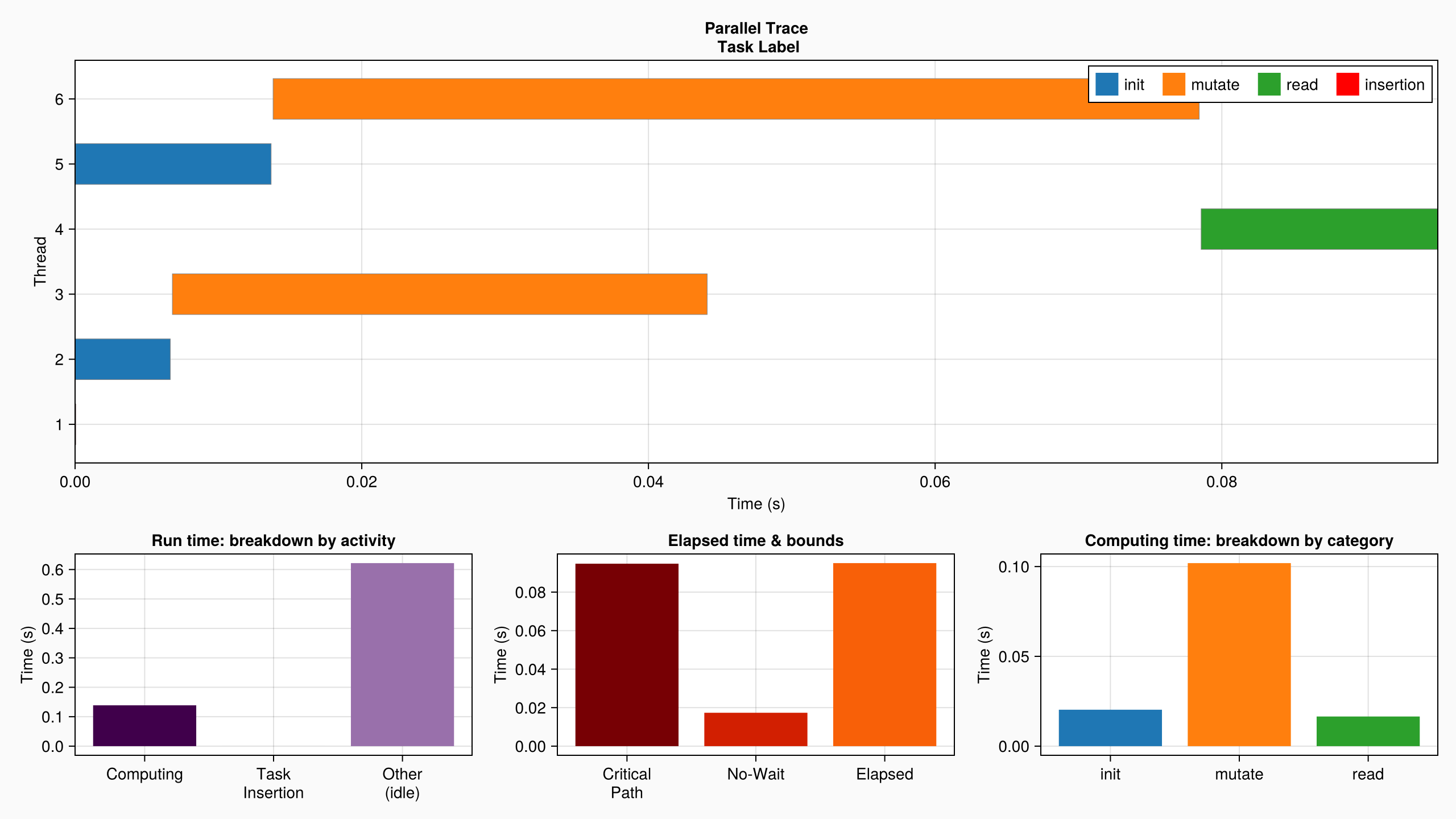

The categories keyword argument allows grouping tasks in categories according to their labels. In the example above, all tasks containing "mutate" in their label will be grouped in the same category.

Note : be careful with giving similar labels. If tasks have "R" and "RW" labels, and the substrings given to the plot's argument are also "R", and "RW", then all tasks will be in the category "R" (because "R" can be found in "RW"). Regular expressions can be given instead of substrings in order to avoid such issues.

Let us explore the various parts of this graph.

Parallel Trace

The main plot (at the top) is the parallel trace visualization. In this example there were two threads; we can see on which thread the task was run, and the time it took.

Even though tasks are grouped in categories by considering substrings in their labels, the full label is shown when hovering over a task in the interactive visualization (i.e. when using GLMakie instead of CairoMakie).

The plot also shows the time spent inserting nodes in the graph (which is part of the overhead incurred by the use of DataFlowTasks): these insertion times are visualized as red tasks. They are not visible for such a small example, but the interactive visualization allows zooming on the plot to search for those small tasks.

Also note that inserting tasks into the graph involves memory allocations, and may thus trigger garbage collector sweeps. When this happens, the time spent in the garbage collector is also shown in the plot.

Run time: breakdown by activity

A barplot in the bottom left corner of the window gives us information on the break-down of parallel run times (summed over all threads):

• Computing represents the total time spent in the tasks bodies (i.e. "useful" work);
• Task Insertion represents the total time spent inserting nodes in the DAG (i.e. overhead induced by DataFlowTasks), possibly including any time spent in the GC if it is triggered by a memory allocation in the task insertion process;
• Other (idle) represents the total idle time on all threads (which may be due to bad scheduling, or simply arise by lack of enough exposed parallelism in the algorithm).

Elapsed time & bounds

A barplot in the bottom center of the window tries to present insightful information about the elapsed (wall-clock) time of the computation, and its limiting factors:

• Elapsed represents the measured "wall clock time" of the computation; it should be larger than both of the bounds described below;

• Critical Path represents the time spent in the longest sequential path in the DAG (shown in red in the DAG visualization). As said above, it bounds the performance in that even infinitely many threads would still have to compute this path sequentially;

• No-Wait represents the duration of a hypothetical computation in which all computing time would be evenly distributed among threads (i.e. no thread would ever have to wait). This also bounds the total time because it does not account for dependencies between tasks.

When looking for faster response times, this graph may suggest sensible ways to explore. If the measured time is close to the critical path duration, then adding more threads will be of no help, but decomposing the work in smaller tasks may be useful. On the other hand, if the measured time is close to the "without waiting" bound, then adding more workers may reduce the wall clock time and scale relatively well.

Computing time: breakdown by category

A barplot in the bottom right of the window displays a break-down of the total computing time (i.e. the total time spent on all threads while performing user-defined tasks), grouped by user-provided category as explained above.

When trying to optimize the sequential performance of the algorithm, this is where one can get data about what actually takes time (and therefore could produce large gains in performance if it could be optimized).