Longest Common Subsequence

The problem of finding the Longest Common Subsequence between two sequences finds numerous applications in fields as diverse as computer sciences or bioinformatics. In this example, we'll implement a parallel dynamic programming approach to solving such problems.

The idea behind this approach is that, if we denote by $LCS(X,Y)$ the longest common subsequence of two sequences $X$ and $Y$, then $LCS$ satisfies the two following properties:

\[\begin{align} & LCS(X*c, Y*c) = LCS(X, Y) * c \\ & LCS(X*c_1, Y*c_2) \in \left\{ LCS(X*c_1, Y), LCS(X, Y*c_2)\right\} & \text{if } c_1 \neq c_2 \end{align}\]

where $X*c$ denotes the concatenation of sequence $X$ with character $c$. The first property above allows simplifying the Longest Common Subsequence computation of two sequences that end with the same character. When the two sequences end with different characters, the second property allows simplifying the problem to a choice between two possibilities.

If we now denote by $L_{i,j}$ the length of the longest common subsequence between the first $i$ characters of $X$ and the first $j$ characters of $Y$, then we now have the following property for $L$:

\[L_{i,j} = \left\{ \begin{array}{ll} 0 & \text{ if } i=0 \text{ or } j=0\\ 1 + L_{i-1, j-1} & \text{ if } i\neq 0 \text{ and } j\neq 0 \text{ and } x_i = y_j\\ \text{max}\left(L_{i-1, j}, L_{i,j-1}\right) & \text{ if } i\neq 0 \text{ and } j\neq 0 \text{ and } x_i \neq y_j\\ \end{array} \right.\]

where $x_i$ represents the $i$-th character in sequence $X$ and $y_j$ the $j$-th character in sequence $Y$.

If $L$ is stored in an array, the first condition above allows initializing its first row and first column. Then, the neighboring cells can be filled using the two other conditions, which in turn unlocks further neighboring cells until the whole $L$ matrix is filled.

Small example

Let us begin with a small example: we want to find a longest common subsequence between GAC and AGCAT:

x = collect("GAC");
y = collect("AGCAT");

Let's build the $L$ array. For the sake of the example, we'll initially fill it with $(-1)$ in order to indicate which values haven't been computed yet. The init_buffer(x,y) function simply initiaizes a buffer matrix L of the appropriate size, while init_length!(L) takes a matrix and fills its first row and first column with zeros. We also define a display helper function, which shows a pretty representation of the $L$ array.

init_buffer(x, y) = Matrix{Int}(undef, 1 + length(x), 1 + length(y))

function init_lengths!(L)
    L[:, 1] .= 0
    return L[1, :] .= 0
end

using PrettyTables
function display(L, x, y)
    return pretty_table(
        hcat(['∅', x...], L);
        header = [' ', '∅', y...],
        formatters = (v, i, j) -> v == -1 ? "" : v,
    )
end

L = fill!(init_buffer(x, y), -1)
init_lengths!(L)
display(L, x, y)

┌───┬───┬───┬───┬───┬───┬───┐
│   │ ∅ │ A │ G │ C │ A │ T │
├───┼───┼───┼───┼───┼───┼───┤
│ ∅ │ 0 │ 0 │ 0 │ 0 │ 0 │ 0 │
│ G │ 0 │   │   │   │   │   │
│ A │ 0 │   │   │   │   │   │
│ C │ 0 │   │   │   │   │   │
└───┴───┴───┴───┴───┴───┴───┘

The fill_lengths! function then allows filling other rows. By default it will fill the entire array, but for the sake of the example we restrict it here to a subset of the rows and/or the columns.

function fill_lengths!(L, x, y, ir = eachindex(x), jr = eachindex(y))
    @inbounds for j in jr, i in ir
        L[i+1, j+1] = (x[i] == y[j]) ? L[i, j] + 1 : max(L[i+1, j], L[i, j+1])
    end
end

fill_lengths!(L, x, y, 1:1)
display(L, x, y)

┌───┬───┬───┬───┬───┬───┬───┐
│   │ ∅ │ A │ G │ C │ A │ T │
├───┼───┼───┼───┼───┼───┼───┤
│ ∅ │ 0 │ 0 │ 0 │ 0 │ 0 │ 0 │
│ G │ 0 │ 0 │ 1 │ 1 │ 1 │ 1 │
│ A │ 0 │   │   │   │   │   │
│ C │ 0 │   │   │   │   │   │
└───┴───┴───┴───┴───┴───┴───┘

After the first row has been filled, we see that $L_{1,1} = 0$ because we can't extract any common subsequence from the first characters in $X$ (G) and $Y$ (A). However, $L_{1,2}=1$ because the first character of $X$ (G) matches the second character of $Y$ (which is also G). In turn this causes all other $L_{1,j}$ values to be equal to 1.

Now that the first row is complete, we can fill the remaining two rows in the array:

fill_lengths!(L, x, y, 2:3)
display(L, x, y)

┌───┬───┬───┬───┬───┬───┬───┐
│   │ ∅ │ A │ G │ C │ A │ T │
├───┼───┼───┼───┼───┼───┼───┤
│ ∅ │ 0 │ 0 │ 0 │ 0 │ 0 │ 0 │
│ G │ 0 │ 0 │ 1 │ 1 │ 1 │ 1 │
│ A │ 0 │ 1 │ 1 │ 1 │ 2 │ 2 │
│ C │ 0 │ 1 │ 1 │ 2 │ 2 │ 2 │
└───┴───┴───┴───┴───┴───┴───┘

We now know that the longest common subsequence between $X$ and $Y$ has a length of 2. In order to actually find a subsequence of this length, we can "backtrack" from the bottom right of the array back to the top left:

function backtrack(L, x, y)
    i = lastindex(x)
    j = lastindex(y)
    subseq = Char[]
    while L[i+1, j+1] != 0
        if x[i] == y[j]
            pushfirst!(subseq, x[i])
            (i, j) = (i - 1, j - 1)
        elseif L[i+1, j] > L[i, j+1]
            (i, j) = (i, j - 1)
        else
            (i, j) = (i - 1, j)
        end
    end
    return String(subseq)
end

backtrack(L, x, y)

"GA"

Wrapping everything into a function, we get

function LCS!(L, x, y)
    init_lengths!(L)
    fill_lengths!(L, x, y)
    return backtrack(L, x, y)
end
LCS(x, y) = LCS!(init_buffer(x, y), x, y)

LCS(x, y)

"GA"

Note that we define both an in-place version of the algorithm, which takes a pre-allocated array as input, and another version which allocates the array internally.

Large example

Let's test this on larger data. The results obtained with this sequential version of the algorithm will serve as reference to check the validity of more complex implementations.

import Random;
Random.seed!(42);
x = rand("ATCG", 4096);
y = rand("ATCG", 8192);
seq = LCS(x, y)
length(seq)

We can also measure the elapsed time for this implementation, which will serve as a base line to assess the performance of other implementations described below.

using BenchmarkTools
BenchmarkTools.DEFAULT_PARAMETERS.seconds = 1
t_seq = @belapsed LCS!(L, $x, $y) setup = (L = init_buffer(x, y))

0.251582155

Tiled sequential version

We'll now build a tiled version of the same algorithm. The TiledIteration.jl package implements various tools allowing to define and iterate over disjoint tiles of a larger array. Among these, the SplitAxis function allows splitting a range of indices into a given number of chunks:

using TiledIteration
SplitAxis(1:20, 3)  # split the range 1:20 into 3 chunks of approximately equal sizes

3-element TiledIteration.SplitAxis:
 1:6
 7:13
 14:20

A tiled version of the previous algorithm is then as simple as filling the chunks one after the other:

function LCS_tiled!(L, x, y, nx, ny)
    init_lengths!(L)
    for jrange in SplitAxis(eachindex(y), ny)
        for irange in SplitAxis(eachindex(x), nx)
            fill_lengths!(L, x, y, irange, jrange)
        end
    end
    return backtrack(L, x, y)
end
LCS_tiled(x, y, nx, ny) = LCS_tiled!(init_buffer(x, y), x, y, nx, ny)

LCS_tiled (generic function with 1 method)

Here we split the problem into $10 \times 10$ blocks, and check that the tiled version gives the same results as the plain implementation above. Even without parallelization, and depending on the characteristics of the system, tiling may already be beneficial in terms of performance because it is more cache-friendly:

nx = ny = 10
tiled = LCS_tiled(x, y, nx, ny)
@assert seq == tiled

t_tiled = @belapsed LCS_tiled!(L, $x, $y, nx, ny) setup = (L = init_buffer(x, y))

0.216198752

Tiling and cache effects

The tiled version of the algorithm above is not exactly equivalent to the sequential version, because the array is visited in a different way when the tiles are used. This can have an impact on the performance, depending on the characteristics of the system and the problem size. In particular, the tiled version may be more cache-friendly, which can lead to better performance even in the absence of parallelization.

Tiled parallel version

Parallelizing the tiled version using DataFlowTasks is now relatively straightforward: it only requires annotating the code to expose data dependencies.

In our case:

the initialization task writes to the first row and first column of the array. In this parallel implementation, initialization will be done tile-by-tile as well using fill! on a view of L;
filling a tile involves reading L for the provided ranges of indices, and writing to a range of indices shifted by 1;
backtracking reads the whole L array.

Note that the backtracking task needs to be fetched in order to get the result in a synchronous way and perform an apple-to-apple comparison to the previous implementations.

using DataFlowTasks

init_lengths!(L, ir, jr) = fill!(view(L, ir, jr), 0)

function LCS_par!(L, x, y, nx, ny)
    L[1,1] = 0
    for (ky, jrange) in enumerate(SplitAxis(eachindex(y), ny))
        L1j = view(L, 1, jrange .+ 1)
        @dspawn fill!(@W(L1j), 0) label = "init (1, $(ky+1))"
        for (kx, irange) in enumerate(SplitAxis(eachindex(x), nx))
            Lx1 = view(L, irange .+ 1, 1)
            ky == 1 && @dspawn fill!(@W(Lx1), 0) label = "init ($(kx+1), 1)"
            @dspawn begin
                @R view(L, irange, jrange)
                @W view(L, irange .+ 1, jrange .+ 1)
                fill_lengths!(L, x, y, irange, jrange)
            end label = "tile ($kx, $ky)"
        end
    end

    bt = @dspawn backtrack(@R(L), x, y) label = "backtrack"
    return fetch(bt)
end
LCS_par(x, y, nx, ny) = LCS_par!(init_buffer(x, y), x, y, nx, ny)

LCS_par (generic function with 1 method)

Again, we can check that this implementation produces the correct results, and measure its run-time.

par = LCS_par(x, y, nx, ny)
@assert seq == par
t_par = @belapsed LCS_par!(L, $x, $y, nx, ny) setup = (L = init_buffer(x, y))

0.081210672

As an added safety measure, let's also check that the task dependency graph looks as expected:

import DataFlowTasks as DFT
resize!(DFT.get_active_taskgraph(), 300)
GC.gc()
log_info = DFT.@log LCS_par(x, y, nx, ny)

DFT.stack_weakdeps_env!()
using GraphViz
dag = GraphViz.Graph(log_info)

Performance comparison

using CairoMakie
barplot(
    1:3,
    [t_seq, t_tiled, t_par];
    axis = (; title = "Run times [s]", xticks = (1:3, ["sequential", "tiled", "parallel"])),
)

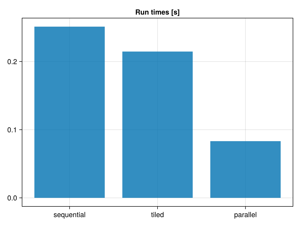
Comparing the performances of these 3 implementations, the tiled version may, depending on the system, already saves some time due to cache effects. The the parallel version does show some speedup, but not as much as one might expect:

(; nthreads = Threads.nthreads(), speedup  = t_seq / t_par)

(nthreads = 8, speedup = 3.097895249530751)

Let's try and understand why. The run-time data collected above contains useful information

DFT.describe(log_info; categories = ["init", "tile", "backtrack"])

• Elapsed time           : 0.101
  ├─ Critical Path       : 0.096
  ╰─ No-Wait             : 0.053

• Run time               : 0.806
  ├─ Computing           :   0.426
  │  ├─ init             :     0.075
  │  ├─ tile             :     0.351
  │  ├─ backtrack        :     0.000
  │  ╰─ unlabeled        :     0.000
  ├─ Task Insertion      :   0.001
  ╰─ Other (idle)        :   0.378

which we can also visualize in a profiling plot. This gives some insight about the performances of our parallel version:

plot(log_info; categories = ["init", "tile", "backtrack"])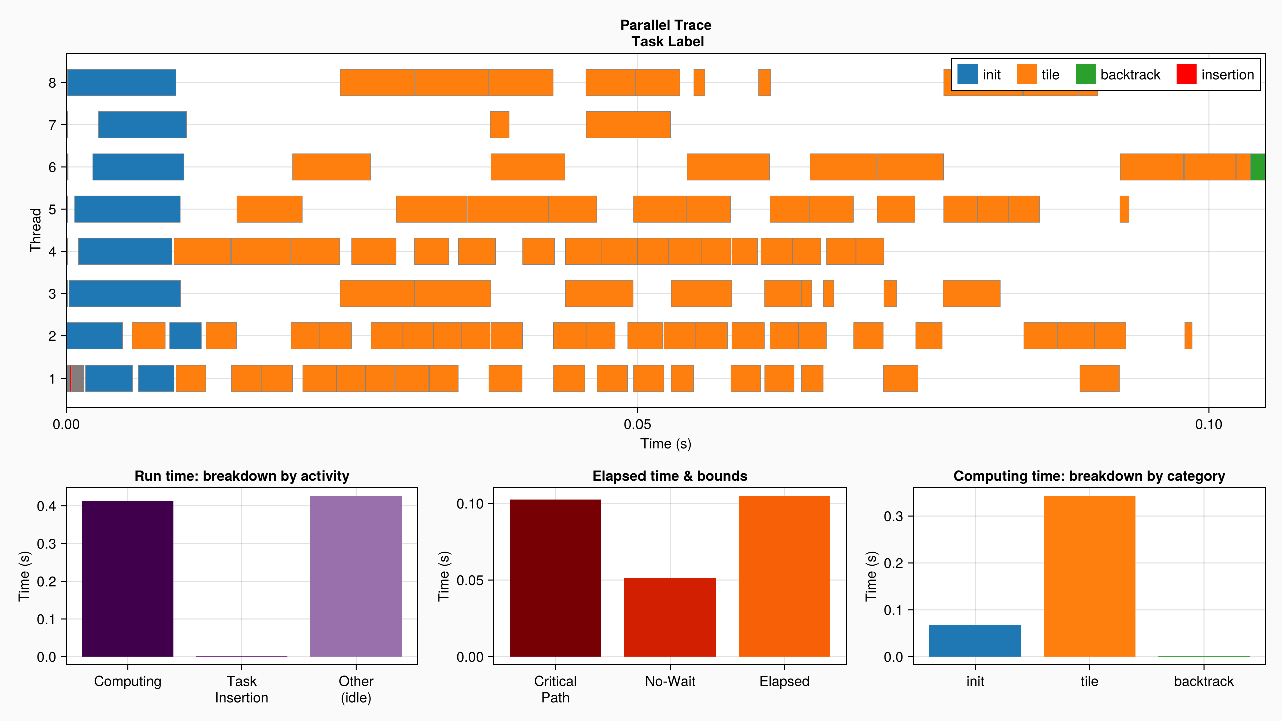

Here, we see for example that the run time is bounded by the length of the critical path, which means that adding more threads would not help much. One way to try and improve the performance is to expose more parallelism by dividing the problem into smaller chunks. Give it a try and see what you get!

This page was generated using Literate.jl.